Plotting Band Structures

%matplotlib inline
# these two lines are only necessary to make the jupyter notebooks run on binder
import sys
sys.path.insert(0, "../..")

# We load the BandStructure class from aimstools
from aimstools import BandStructure

# We initialize this class from results in the directory "bandstructure"
bs = BandStructure("bandstructure")

# The BandStructure class is only a wrapper that gives you easy access to the underlying classes.
# You can access an information overview with:
bs.get_properties()

# The plot() method is a quick way to visualize everything, but cannot be customized as much.
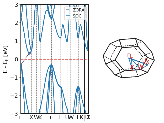
bs.plot()

INFO     Analyzing RegularBandStructure(outputfile=PosixPath('bandstructure/aims.out'),
         spin_orbit_coupling=True) ...

INFO     The band structure has been calculated with spin-orbit-coupling.

INFO     The band gap from the output file is 0.6213 eV large.

INFO     From the spectrum, the fundamental band gap is 0.62133 eV large and indirect.

INFO     The VBM is located at k = ( 0.0000 0.0000 0.0000 ) in units of the reciprocal
         lattice.

INFO     The CBM is located at k = ( 0.4167 -0.0000 0.4167 ) in units of the reciprocal
         lattice.

INFO     The smallest direct band gap is 2.5184 eV large and is located at k = ( 0.0000
         0.0000 0.0000 ) in units of the reciprocal lattice.

INFO     Plotting regular band structure with ZORA+SOC.

[<AxesSubplot:ylabel='E - E$_{\\mathrm{F}}$ [eV]'>, <Axes3DSubplot:>]

# If you want to customize the plot, you need to access the subclasses where the information is actually stored:
bs_zora = bs.regular_bandstructure_zora
bs_soc = bs.regular_bandstructure_soc

# ZORA and SOC band structures are typically overlaid. This can easily be done this way:
import matplotlib.pyplot as plt
from matplotlib.lines import Line2D

fig, axes = plt.subplots(1,1, figsize=(5,5))
# The main attribute specifies which plot is the most important one, such that gridlines and
# the Fermi level are only drawn once. In many cases, this option is not needed.
axes = bs_zora.plot(axes=axes, color="gray", alpha=0.5, main=False)
axes = bs_soc.plot(axes=axes, color="royalblue", main=True, linestyle=":")
handles = []
handles.append(Line2D([0], [0], color="gray", label="ZORA", lw=1.5))
handles.append(Line2D([0], [0], color="royalblue", label="ZORA+SOC", lw=1.5))
lgd = axes.legend(
    handles=handles,
    frameon=True,
    fancybox=False,
    borderpad=0.4,
    loc="upper right",
)
plt.show()

# The band structure objects have a lot of possible arguments. To summarize:

#            axes (matplotlib.axes.Axes): Axes to draw on, defaults to None.
#            figsize (tuple): Figure size in inches. Defaults to (5,5).
#            filename (str): Saves figure to file. Defaults to None.
#            spin (int): Spin channel, can be "up", "dn", 0 or 1. Defaults to 0.
#            bandpath (str): Band path for plotting of form "GMK,GA".
#            reference (str): Energy reference for plotting, e.g., "VBM", "middle", "fermi level". Defaults to None.
#            show_fermi_level (bool): Show Fermi level. Defaults to True.
#            fermi_level_color (str): Color of Fermi level line. Defaults to fermi_color.
#            fermi_level_alpha (float): Alpha channel of Fermi level line. Defaults to 1.0.
#            fermi_level_linestyle (str): Line style of Fermi level line. Defaults to "--".
#            fermi_level_linewidth (float): Line width of Fermi level line. Defaults to mpllinewidth.
#            show_grid_lines (bool): Show grid lines for axes ticks. Defaults to True.
#            grid_lines_axes (str): Show grid lines for given axes. Defaults to "x".
#            grid_linestyle (tuple): Grid lines linestyle. Defaults to (0, (1, 1)).
#            grid_linewidth (float): Width of grid lines. Defaults to 1.0.
#            show_jumps (bool): Show jumps between Brillouin zone sections by darker vertical lines. Defaults to True.
#            jumps_linewidth (float): Width of jump lines. Defaults to mpllinewidth.
#            jumps_linestyle (str): Line style of the jump lines. Defaults to "-".
#            jumps_linecolor (str): Color of the jump lines. Defaults to mutedblack.
#            show_bandstructure (bool): Show band structure lines. Defaults to True.
#            bands_color (bool): Color of the band structure lines. Synonymous with color. Defaults to mutedblack.
#            bands_linewidth (float): Line width of band structure lines. Synonymous with linewidth. Defaults to mpllinewidth.
#            bands_linestyle (str): Band structure lines linestyle. Synonymous with linestyle. Defaults to "-".
#            bands_alpha (float): Band structure lines alpha channel. Synonymous with alpha. Defaults to 1.0.
#            show_bandgap_vertices (bool): Show direct and indirect band gap transitions. Defaults to True.
#            window (tuple): Window on energy axis, can be float or tuple of two floats in eV. Defaults to 3 eV.
#            y_tick_locator (float): Places ticks on energy axis on regular intervals. Defaults to 0.5 eV.


# For example:
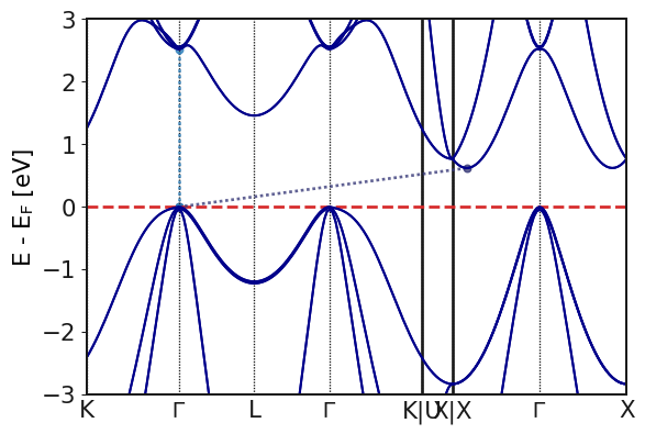
axes = bs_soc.plot(figsize = (6,4),
            color="darkblue",
            linewidth=1.5,
            bandpath="KGLGK,UX,XGX",
            reference="VBM")
plt.show()

%matplotlib inline

# The most common task is to show bandstructures and densities of states side by side.
# With these tools, that is very easy:

from aimstools.bandstructures import RegularBandStructure
from aimstools.density_of_states import SpeciesProjectedDOS

bs1 = RegularBandStructure("bandstructure", soc=False)
bs2 = RegularBandStructure("bandstructure", soc=True)
dos = SpeciesProjectedDOS("bandstructure", soc=True)

import matplotlib.pyplot as plt
from matplotlib import gridspec

fig = plt.figure(constrained_layout=True, figsize=(8, 6))
spec = gridspec.GridSpec(ncols=2, nrows=1, figure=fig, width_ratios=[3, 1])

ax1 = fig.add_subplot(spec[0])
ax1 = bs1.plot(axes=ax1, color="gray", main=False)
ax1 = bs2.plot(axes=ax1, color="royalblue", main=True)

# The options to plot DOS are discussed in another tutorial. Here, we just plot all species.
ax2 = fig.add_subplot(spec[1])
ax2 = dos.plot_all_species(axes=ax2)

ax2.set_yticks([])
ax2.set_ylabel("")
fig.suptitle("Band structure + DOS")
plt.show()